Geometric Distribution Formula, Explanation, Derivation, Examples

Geometric Distribution Formula: Geometric Distribution is one of the most important concepts related to the world of probability. It is used in the case of discrete probability. This formula is associated with the concept of the Bernoulli Trial. It is applied when there is a constant chance of success across all trials and each experiment has the potential to succeed or fail. In this scenario, this formula is used to calculate the chances of success or failure. Let us understand the geometric distribution formula concept in more detail by understanding its different aspects.

Meaning of Geometric Distribution

Before exploring the Geometric Distribution Formula, let us first understand what is Geometric Distribution. Geometric Distribution is a Discrete Probability Distribution that is used to find the probability of success of an event when there are two outcomes of an event. The likelihood of the number of consecutive failures before success is attained in a Bernoulli trial is represented by a geometric distribution. In other words, in a series of independent Bernoulli trials with a fixed probability of success, the geometric distribution gives us the probability distribution that represents the number of trials necessary to reach the first success. A Bernoulli Trial is is an experiment that can only result in one of two outcomes, either success or failure. In a geometric distribution, a Bernoulli trial is essentially repeated until success is achieved and at that point point, the trial is halted. After knowing the meaning of Geometric Distribution, let us understand its formula.

Geometric Distribution Formula

As mentioned earlier, a geometric distribution can be used to describe the likelihood of experiencing success for the first time following a string of failures. Up until the first success, a geometric distribution can undergo an infinite number of trials. The geometric distribution can take two different discrete probability distribution:

1. The probability distribution of the number X of successful Bernoulli trials over the set {1, 2, 3, ……..}. These distributions can be represented byP (X = n) = p(1-p)^n-1, where n = 1, 2, 3,…..P (n) = 0, for all other cases
2. The probability distribution of the number Y = X-1 of failed Bernoulli trials before the first success over the set {0, 1, 2, 3, ……..}. These distributions can be represented byP (X = n) = p(1-p)ⁿ, where n = 0, 1, 2, 3,…..P (n) = 0, for all other cases

We can derive the general formula for the geometric distribution.

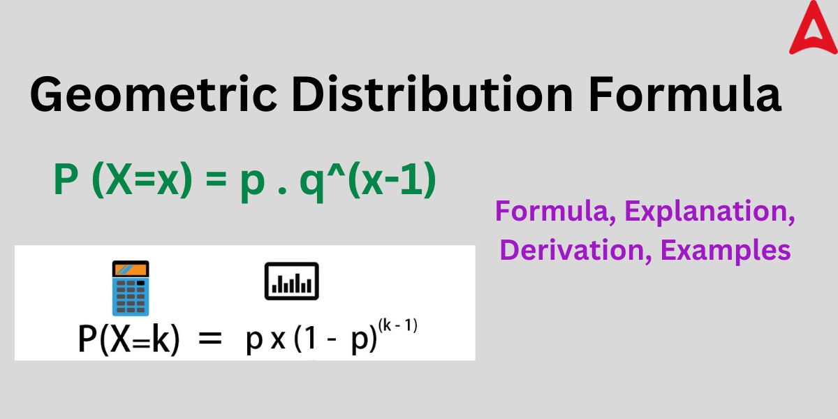
The geometric distribution formula is given by:

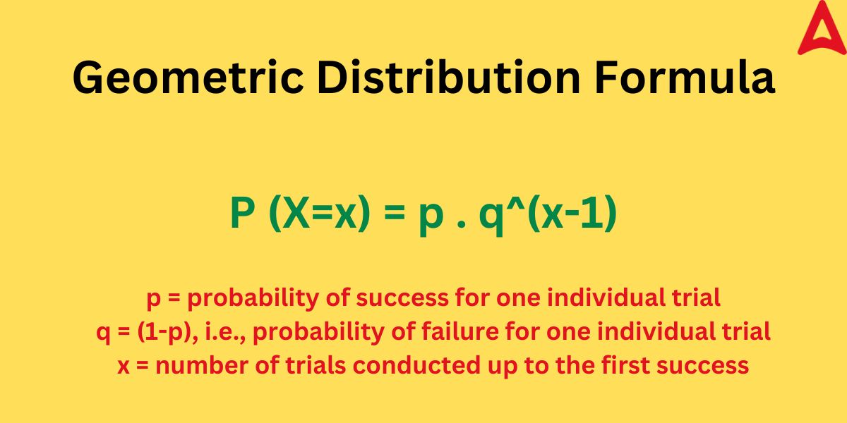
P (X = x) = p . q^{(x – 1)}, for x = 1, 2, 3, 4, ……….

p = probability of success for one individual trial

q = (1-p), i.e., probability of failure for one individual trial

x = number of trials conducted up to the first success

Geometric Distribution PMF and CDF Formula

The probability mass function (PMF) estimates the possibility that a discrete random variable, X, would exactly match a given value, x. The Geometric Distribution formula for PMF is given by:

P(X = x) = p(1 – p)^{x -1}

p = probability of success for one individual trial

(1-p) = probability of failure for one individual trial

The cumulative distribution function (CDF) of a random variable, X, that is evaluated at a point, x, can be used to characterize the likelihood that a random variable, X, would assume a value that is less than or equal to x.

P(X ≤ x) = 1 – (1 – p)^x

Geometric Distribution Formula Assumptions

The geometric distribution formula can be applied on a certain trial if and only if it satisfies the following assumptions:

• Each trial must be independent
• There must be only two outcomes of a trial: success or failure
• The probability of success or failure for each independent trial must be constant

If any experiment does not satisfies the assumptions mentioned above, then the geometric distribution formula cannot be applied.

Geometric Distribution Formula for Mean

We can find the mean of the number of trials in a Bernoulli experiment. The geometric distribution formula for mean is given by:

E[X] = 1 / p

where E[X] = mean value

p = probability of success of the individual trial

Geometric Distribution Expected Value Formula

The expected value of the geometric distribution is equal to its mean. The expected value of a random variable, X, is the weighted average of all of its values. So, the geometric distribution formula for the expected value is given by:

E[X] = 1 / p

Geometric Distribution Formula for Variance

A measure of dispersion called variance looks at how far data in a distribution deviate from the mean. The geometric distribution formula for the variance is given by:

Var[X] = (1 – p) / p²

where Var[X] = variance

Geometric Distribution Formula for Standard Deviation

As we know that the standard deviation can be calculated by taking the square root of the variance. The distribution’s divergence from the mean is depicted by the standard deviation. The geometric distribution formula for the standard deviation is given by:

S.D[X] = √VAR[X]

S.D[X] = √1-p / p

Geometric Distribution Formula Derivation

we can find out the derivation for the variance formula of the geometric distribution. The proof of the geometric distribution formula for the variance is given below:

As we know variance = expected values of squared observations – square of expected value

i.e., Var[X] = E(X²) – (E(X))²  ———- (i)

we know that the expectation of the function of discrete random variable x is given by

E(X²) =

² . P(X=x)

as geometric probability distribution mandates that  p = 1-q, such that p + q = 1

where, p = probability of success of individual trial

q = probability of failure of individual trial

using these values and simplifying the equation, we get:

E(X²) =

k².q.p^k

or, E(X²) = p

k².q.p^k-1

Using the rule of shifted geometric distribution, we get

E(X²) = p [(2/q²) -(1/q)]

as E(X) = 1/p

so, (E(X))² = 1/p²

putting the values of E(X²) and (E(X))² in equation (i), we get:

Var[X] = (1-p)/p²

Hence, proved

Geometric Distribution Formula Examples

Some of the solved examples on this topic is given below so that students can get a clear understanding of this concept.

Example 1: Find the anticipated number of donors who will be tested up until a match is found, including the matched donor, if a patient is waiting for a suitable blood donor and the likelihood that the selected donor will be a match is 0.2.

Solution: As we have been given p (success of matching) = 0.2

we have to find the expected number, i.e., the mean

As E(X) = 1/p, where E(X) = mean

so E(X) = 1/0.2

E(X) = 5

so, the expected numbers of donors that will be tested until a successful match = 5

Example 2: Imagine you are participating in a darts game. There is a 0.4 chance of success. What is the likelihood that your second attempt will result in a successful bullseye?

Solution: Given the probability of success p = 0.4

so, probability of failure q = 1 – p = 0.6

given the attempt value (x) = 2

By using the geometric distribution formula of P (X=x) = p . q^{(x – 1)}

P (X=2) = (0.4) x (0.6)^2-1

P (X=2) = 0.4 x 0.6

P(X=2) = 0.24

Hence, the probability that the second attempt will result in a bull’s eye = 0.24

Example 3: If the mean of a geometric distribution is given to be 2. Find out its variance.

Solution: given mean = 2

As we know that mean = 1/p

so, 2 = 1/p

or, p = 1/2

p = 0.5

standard deviation of a geometric distribution is given by:

S.D. = (1-p)/p²

S.D. = (1-0.5)/(0.5)²

S.D. = 0.5/(0.5)²

or, S.D. = 1/0.5

Hence, standard deviation = 2

Sharing is caring!