A teacher has created a spreadsheet of test marks of five students. She has written a formula HLOOKUP(B4, $D$1: $K$2, 2) in cell C4 and copies this formula from cell c4 to the range C5 : C8. What values will be returned by the formulae in the range C4 : C8?

Correct option is D

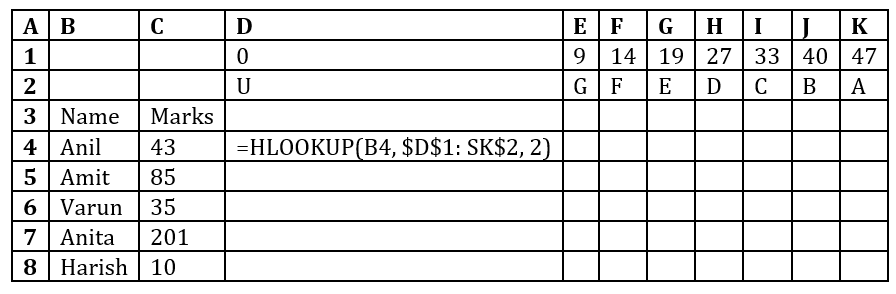
Formula: =HLOOKUP(B4, $D$1: $K$2, 2)
Range: C4 : C8
The HLOOKUP function searches for the value in B4 (in this case, 43) in the first row of the range $D$1:$K$2 and returns the corresponding value from the second row. Since the formula is copied down, the marks in each row (e.g., B5, B6) will be searched in the first row of the range, and the matching second-row value will be returned.
Values returned:
1. C4: B
2. C5: A
3. C6: C
4. C7: E
5. C8: G